12.13. Image Classification (CIFAR-10) on Kaggle¶

So far, we have been using Gluon’s data package to directly obtain image data sets in NDArray format. In practice, however, image data sets often exist in the format of image files. In this section, we will start with the original image files and organize, read, and convert the files to NDArray format step by step.

We performed an experiment on the CIFAR-10 data set in Section 12.1. This is an important data set in the computer vision field. Now, we will apply the knowledge we learned in the previous sections in order to participate in the Kaggle competition, which addresses CIFAR-10 image classification problems. The competition’s web address is

https://www.kaggle.com/c/cifar-10

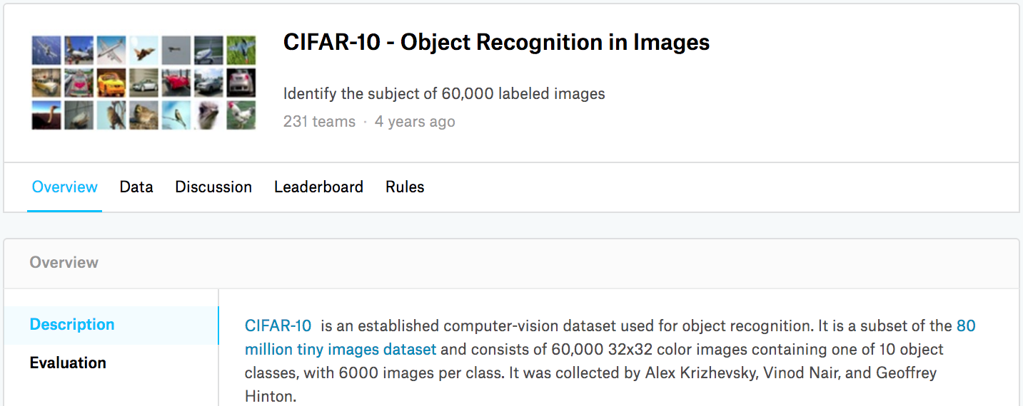
Figure 11.16 shows the information on the competition’s webpage. In order to submit the results, please register an account on the Kaggle website first.

Fig. 12.13.1 CIFAR-10 image classification competition webpage information. The data set for the competition can be accessed by clicking the “Data” tab.

First, import the packages or modules required for the competition.

import d2l
from mxnet import autograd, gluon, init
from mxnet.gluon import nn
import os
import pandas as pd
import shutil
import time

12.13.1. Obtain and Organize the Data Sets¶

The competition data is divided into a training set and testing set. The training set contains 50,000 images. The testing set contains 300,000 images, of which 10,000 images are used for scoring, while the other 290,000 non-scoring images are included to prevent the manual labeling of the testing set and the submission of labeling results. The image formats in both data sets are PNG, with heights and widths of 32 pixels and three color channels (RGB). The images cover 10 categories: planes, cars, birds, cats, deer, dogs, frogs, horses, boats, and trucks. The upper-left corner of Figure 11.16 shows some images of planes, cars, and birds in the data set.

12.13.1.1. Download the Data Set¶

After logging in to Kaggle, we can click on the “Data” tab on the CIFAR-10 image classification competition webpage shown in Figure 11.16 and download the training data set “train.7z”, the testing data set “test.7z”, and the training data set labels “trainlabels.csv”.

12.13.1.2. Unzip the Data Set¶

The training data set “train.7z” and the test data set “test.7z” need to be unzipped after downloading. After unzipping the data sets, store the training data set, test data set, and training data set labels in the following respective paths:

../data/kaggle_cifar10/train/[1-50000].png
../data/kaggle_cifar10/test/[1-300000].png
../data/kaggle_cifar10/trainLabels.csv

To make it easier to get started, we provide a small-scale sample of the data set mentioned above. “train_tiny.zip” contains 100 training examples, while “test_tiny.zip” contains only one test example. Their unzipped folder names are “train_tiny” and “test_tiny”, respectively. In addition, unzip the zip file of the training data set labels to obtain the file “trainlabels.csv”. If you are going to use the full data set of the Kaggle competition, you will also need to change the following demo variable to False.

# If you use the full data set downloaded for the Kaggle competition, change
# the demo variable to False
demo = True
if demo:
    import zipfile
    for f in ['train_tiny.zip', 'test_tiny.zip', 'trainLabels.csv.zip']:
        with zipfile.ZipFile('../data/kaggle_cifar10/' + f, 'r') as z:
            z.extractall('../data/kaggle_cifar10/')

12.13.1.3. Organize the Data Set¶

We need to organize data sets to facilitate model training and testing. The following read_label_file function will be used to read the label file for the training data set. The parameter valid_ratio in this function is the ratio of the number of examples in the validation set to the number of examples in the original training set.

def read_label_file(data_dir, label_file, train_dir, valid_ratio):
    with open(os.path.join(data_dir, label_file), 'r') as f:
        # Skip the file header line (column name)
        lines = f.readlines()[1:]
        tokens = [l.rstrip().split(',') for l in lines]
        idx_label = dict(((int(idx), label) for idx, label in tokens))
    labels = set(idx_label.values())
    n_train_valid = len(os.listdir(os.path.join(data_dir, train_dir)))
    n_train = int(n_train_valid * (1 - valid_ratio))
    assert 0 < n_train < n_train_valid
    return n_train // len(labels), idx_label

Below we define a helper function to create a path only if the path does not already exist.

# save to the d2l package.
def mkdir_if_not_exist(path):
    if not os.path.exists(os.path.join(*path)):
        os.makedirs(os.path.join(*path))

Next, we define the reorg_train_valid function to segment the validation set from the original training set. Here, we use valid_ratio=0.1 as an example. Since the original training set has 50,000 images, there will be 45,000 images used for training and stored in the path “input_dir/train” when tuning hyper-parameters, while the other 5,000 images will be stored as validation set in the path “input_dir/valid”. After organizing the data, images of the same type will be placed under the same folder so that we can read them later.

def reorg_train_valid(data_dir, train_dir, input_dir, n_train_per_label,
                      idx_label):
    label_count = {}
    for train_file in os.listdir(os.path.join(data_dir, train_dir)):
        idx = int(train_file.split('.')[0])
        label = idx_label[idx]
        mkdir_if_not_exist([data_dir, input_dir, 'train_valid', label])
        shutil.copy(os.path.join(data_dir, train_dir, train_file),
                    os.path.join(data_dir, input_dir, 'train_valid', label))
        if label not in label_count or label_count[label] < n_train_per_label:
            mkdir_if_not_exist([data_dir, input_dir, 'train', label])
            shutil.copy(os.path.join(data_dir, train_dir, train_file),
                        os.path.join(data_dir, input_dir, 'train', label))
            label_count[label] = label_count.get(label, 0) + 1
        else:
            mkdir_if_not_exist([data_dir, input_dir, 'valid', label])
            shutil.copy(os.path.join(data_dir, train_dir, train_file),
                        os.path.join(data_dir, input_dir, 'valid', label))

The reorg_test function below is used to organize the testing set to facilitate the reading during prediction.

def reorg_test(data_dir, test_dir, input_dir):
    mkdir_if_not_exist([data_dir, input_dir, 'test', 'unknown'])
    for test_file in os.listdir(os.path.join(data_dir, test_dir)):
        shutil.copy(os.path.join(data_dir, test_dir, test_file),
                    os.path.join(data_dir, input_dir, 'test', 'unknown'))

Finally, we use a function to call the previously defined reorg_test, reorg_train_valid, and reorg_test functions.

def reorg_cifar10_data(data_dir, label_file, train_dir, test_dir, input_dir,
                       valid_ratio):
    n_train_per_label, idx_label = read_label_file(data_dir, label_file,
                                                   train_dir, valid_ratio)
    reorg_train_valid(data_dir, train_dir, input_dir, n_train_per_label,
                      idx_label)
    reorg_test(data_dir, test_dir, input_dir)

We use only 100 training example and one test example here. The folder names for the training and testing data sets are “train_tiny” and “test_tiny”, respectively. Accordingly, we only set the batch size to 1. During actual training and testing, the complete data set of the Kaggle competition should be used and batch_size should be set to a larger integer, such as 128. We use 10% of the training examples as the validation set for tuning hyper-parameters.

if demo:
    # Note: Here, we use small training sets and small testing sets and the
    # batch size should be set smaller. When using the complete data set for
    # the Kaggle competition, the batch size can be set to a large integer
    train_dir, test_dir, batch_size = 'train_tiny', 'test_tiny', 1
else:
    train_dir, test_dir, batch_size = 'train', 'test', 128
data_dir, label_file = '../data/kaggle_cifar10', 'trainLabels.csv'
input_dir, valid_ratio = 'train_valid_test', 0.1
reorg_cifar10_data(data_dir, label_file, train_dir, test_dir, input_dir,
                   valid_ratio)

12.13.2. Image Augmentation¶

To cope with overfitting, we use image augmentation. For example, by adding transforms.RandomFlipLeftRight(), the images can be flipped at random. We can also perform normalization for the three RGB channels of color images using transforms.Normalize(). Below, we list some of these operations that you can choose to use or modify depending on requirements.

transform_train = gluon.data.vision.transforms.Compose([
    # Magnify the image to a square of 40 pixels in both height and width
    gluon.data.vision.transforms.Resize(40),
    # Randomly crop a square image of 40 pixels in both height and width to
    # produce a small square of 0.64 to 1 times the area of the original
    # image, and then shrink it to a square of 32 pixels in both height and
    # width
    gluon.data.vision.transforms.RandomResizedCrop(32, scale=(0.64, 1.0),
                                              ratio=(1.0, 1.0)),
    gluon.data.vision.transforms.RandomFlipLeftRight(),
    gluon.data.vision.transforms.ToTensor(),
    # Normalize each channel of the image
    gluon.data.vision.transforms.Normalize([0.4914, 0.4822, 0.4465],
                                      [0.2023, 0.1994, 0.2010])])

In order to ensure the certainty of the output during testing, we only perform normalization on the image.

transform_test = gluon.data.vision.transforms.Compose([
    gluon.data.vision.transforms.ToTensor(),
    gluon.data.vision.transforms.Normalize([0.4914, 0.4822, 0.4465],
                                      [0.2023, 0.1994, 0.2010])])

12.13.3. Read the Data Set¶

Next, we can create the ImageFolderDataset instance to read the organized data set containing the original image files, where each data instance includes the image and label.

# Read the original image file. Flag=1 indicates that the input image has
# three channels (color)
train_ds = gluon.data.vision.ImageFolderDataset(
    os.path.join(data_dir, input_dir, 'train'), flag=1)
valid_ds = gluon.data.vision.ImageFolderDataset(
    os.path.join(data_dir, input_dir, 'valid'), flag=1)
train_valid_ds = gluon.data.vision.ImageFolderDataset(
    os.path.join(data_dir, input_dir, 'train_valid'), flag=1)
test_ds = gluon.data.vision.ImageFolderDataset(
    os.path.join(data_dir, input_dir, 'test'), flag=1)

We specify the defined image augmentation operation in DataLoader. During training, we only use the validation set to evaluate the model, so we need to ensure the certainty of the output. During prediction, we will train the model on the combined training set and validation set to make full use of all labelled data.

train_iter = gluon.data.DataLoader(train_ds.transform_first(transform_train),
                              batch_size, shuffle=True, last_batch='keep')
valid_iter = gluon.data.DataLoader(valid_ds.transform_first(transform_test),
                              batch_size, shuffle=True, last_batch='keep')
train_valid_iter = gluon.data.DataLoader(train_valid_ds.transform_first(
    transform_train), batch_size, shuffle=True, last_batch='keep')
test_iter = gluon.data.DataLoader(test_ds.transform_first(transform_test),
                             batch_size, shuffle=False, last_batch='keep')

12.13.4. Define the Model¶

Here, we build the residual blocks based on the HybridBlock class, which is slightly different than the implementation described in Section 7.6. This is done to improve execution efficiency.

class Residual(nn.HybridBlock):
    def __init__(self, num_channels, use_1x1conv=False, strides=1, **kwargs):
        super(Residual, self).__init__(**kwargs)
        self.conv1 = nn.Conv2D(num_channels, kernel_size=3, padding=1,
                               strides=strides)
        self.conv2 = nn.Conv2D(num_channels, kernel_size=3, padding=1)
        if use_1x1conv:
            self.conv3 = nn.Conv2D(num_channels, kernel_size=1,
                                   strides=strides)
        else:
            self.conv3 = None
        self.bn1 = nn.BatchNorm()
        self.bn2 = nn.BatchNorm()

    def hybrid_forward(self, F, X):
        Y = F.relu(self.bn1(self.conv1(X)))
        Y = self.bn2(self.conv2(Y))
        if self.conv3:
            X = self.conv3(X)
        return F.relu(Y + X)

Next, we define the ResNet-18 model.

def resnet18(num_classes):
    net = nn.HybridSequential()
    net.add(nn.Conv2D(64, kernel_size=3, strides=1, padding=1),
            nn.BatchNorm(), nn.Activation('relu'))

    def resnet_block(num_channels, num_residuals, first_block=False):
        blk = nn.HybridSequential()
        for i in range(num_residuals):
            if i == 0 and not first_block:
                blk.add(Residual(num_channels, use_1x1conv=True, strides=2))
            else:
                blk.add(Residual(num_channels))
        return blk

    net.add(resnet_block(64, 2, first_block=True),
            resnet_block(128, 2),
            resnet_block(256, 2),
            resnet_block(512, 2))
    net.add(nn.GlobalAvgPool2D(), nn.Dense(num_classes))
    return net

The CIFAR-10 image classification challenge uses 10 categories. We will perform Xavier random initialization on the model before training begins.

def get_net(ctx):
    num_classes = 10
    net = resnet18(num_classes)
    net.initialize(ctx=ctx, init=init.Xavier())
    return net

loss = gluon.loss.SoftmaxCrossEntropyLoss()

12.13.5. Define the Training Functions¶

We will select the model and tune hyper-parameters according to the model’s performance on the validation set. Next, we define the model training function train. We record the training time of each epoch, which helps us compare the time costs of different models.

def train(net, train_iter, valid_iter, num_epochs, lr, wd, ctx, lr_period,
          lr_decay):
    trainer = gluon.Trainer(net.collect_params(), 'sgd',
                            {'learning_rate': lr, 'momentum': 0.9, 'wd': wd})
    for epoch in range(num_epochs):
        train_l_sum, train_acc_sum, n, start = 0.0, 0.0, 0, time.time()
        if epoch > 0 and epoch % lr_period == 0:
            trainer.set_learning_rate(trainer.learning_rate * lr_decay)
        for X, y in train_iter:
            y = y.astype('float32').as_in_context(ctx)
            with autograd.record():
                y_hat = net(X.as_in_context(ctx))
                l = loss(y_hat, y).sum()
            l.backward()
            trainer.step(batch_size)
            train_l_sum += l.asscalar()
            train_acc_sum += (y_hat.argmax(axis=1) == y).sum().asscalar()
            n += y.size
        time_s = "time %.2f sec" % (time.time() - start)
        if valid_iter is not None:
            valid_acc = d2l.evaluate_accuracy_gpu(net, valid_iter)
            epoch_s = ("epoch %d, loss %f, train acc %f, valid acc %f, "
                       % (epoch + 1, train_l_sum / n, train_acc_sum / n,
                       valid_acc))
        else:
            epoch_s = ("epoch %d, loss %f, train acc %f, " %
                       (epoch + 1, train_l_sum / n, train_acc_sum / n))
        print(epoch_s + time_s + ', lr ' + str(trainer.learning_rate))

12.13.6. Train and Validate the Model¶

Now, we can train and validate the model. The following hyper-parameters can be tuned. For example, we can increase the number of epochs. Because lr_period and lr_decay are set to 80 and 0.1 respectively, the learning rate of the optimization algorithm will be multiplied by 0.1 after every 80 epochs. For simplicity, we only train one epoch here.

ctx, num_epochs, lr, wd = d2l.try_gpu(), 1, 0.1, 5e-4
lr_period, lr_decay, net = 80, 0.1, get_net(ctx)
net.hybridize()
train(net, train_iter, valid_iter, num_epochs, lr, wd, ctx, lr_period,
      lr_decay)

epoch 1, loss 6.033371, train acc 0.055556, valid acc 0.100000, time 1.28 sec, lr 0.1

12.13.7. Classify the Testing Set and Submit Results on Kaggle¶

After obtaining a satisfactory model design and hyper-parameters, we use all training data sets (including validation sets) to retrain the model and classify the testing set.

net, preds = get_net(ctx), []
net.hybridize()
train(net, train_valid_iter, None, num_epochs, lr, wd, ctx, lr_period,
      lr_decay)

for X, _ in test_iter:
    y_hat = net(X.as_in_context(ctx))
    preds.extend(y_hat.argmax(axis=1).astype(int).asnumpy())
sorted_ids = list(range(1, len(test_ds) + 1))
sorted_ids.sort(key=lambda x: str(x))
df = pd.DataFrame({'id': sorted_ids, 'label': preds})
df['label'] = df['label'].apply(lambda x: train_valid_ds.synsets[x])
df.to_csv('submission.csv', index=False)

epoch 1, loss 6.466181, train acc 0.100000, time 1.16 sec, lr 0.1

After executing the above code, we will get a “submission.csv” file. The format of this file is consistent with the Kaggle competition requirements. The method for submitting results is similar to method in Section 4.10.

12.13.8. Summary¶

We can create an ImageFolderDataset instance to read the data set containing the original image files.
We can use convolutional neural networks, image augmentation, and hybrid programming to take part in an image classification competition.

12.13.9. Exercises¶

Use the complete CIFAF-10 data set for the Kaggle competition. Change the batch_size and number of epochs num_epochs to 128 and 100, respectively. See what accuracy and ranking you can achieve in this competition.
What accuracy can you achieve when not using image augmentation?
Scan the QR code to access the relevant discussions and exchange ideas about the methods used and the results obtained with the community. Can you come up with any better techniques?